Evidence & Methods
Before trusting a forecast, ask whether it beat last month’s number
Looking back from September 9, 2026, 55 of 111 published forecast series beat carry-forward across six matched one-step observations. Only 25 won in both three-observation halves.
Editorial evidence cutoff: September 9, 2026. Published September 29, 2026. Observation periods are stated throughout; older figures are retrospective evidence.
Before a manufacturer builds a September 2026 budget around a forecast chart, one backward-looking question deserves an answer: did the model beat simply reusing the previous month’s number? A forecast can land close to the outcome and still add little to a decision. Manufacturing industrial production provides a precise example. In the saved MFG Calcs evaluation, the model's displayed average percentage error was just 1.50%. Yet across the six evaluated months, simply predicting that next month's index would equal the latest month's value produced substantially smaller errors.
We applied that same comparison to every published forecast with six usable evaluation observations. Of 111 series, 55 beat the carry-forward benchmark on mean absolute error. The other 56 did not. The median model-to-benchmark error ratio was approximately 1.00: the middle series performed almost identically to the simple alternative, with a slightly larger error before rounding. This short retrospective evaluation shows why an accuracy score needs a benchmark. It cannot establish next year’s performance.
View full-size chart
Scroll horizontally to read every label. Keyboard users can focus the chart area and use the arrow keys.
THE EASY FORECAST IS A SERIOUS OPPONENT
The benchmark has one rule: use the previous calendar month's observed value as the prediction for the next month. It requires no estimated trend, no seasonal parameters and no explanation of the latest economic news. Its value is that it exposes how much apparent accuracy comes from the fact that many economic series change only a little between adjacent months.
We compared that rule with the model on the same actual outcomes, one series at a time. For each prediction, we took the absolute difference from the outcome and averaged the six errors. A model-to-benchmark ratio below one means the model improved on carry-forward. A ratio above one means the benchmark did better. We did not add errors measured in dollars, index points and thousands of jobs into one meaningless total.
This is a one-month-ahead comparison. The site's evaluation code trains on earlier observations and makes each held-out prediction one step forward; the final evaluation segment is separate from parameter selection and interval calibration. Matching the benchmark to that horizon is essential. None of the findings here grades the full six-month forecast path or the coverage of its uncertainty bands. Forecast evaluation guidance likewise distinguishes the error measure from the question of whether a forecasting method improves on an appropriate reference.
PRODUCTION EXPOSES THE MISSING COMPARISON
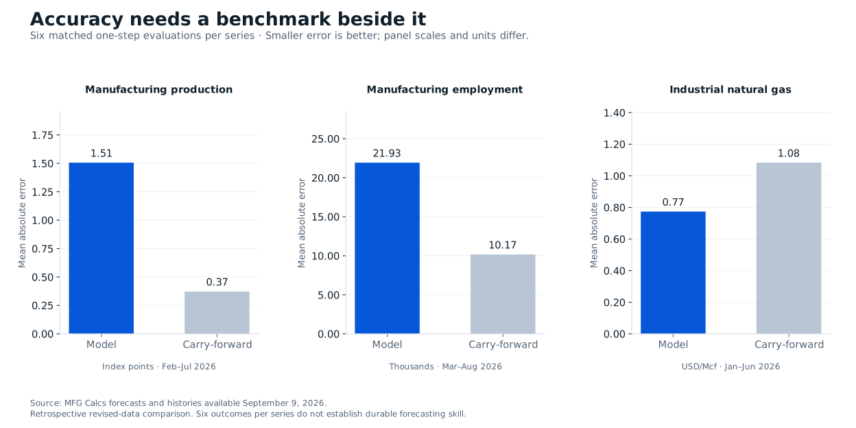
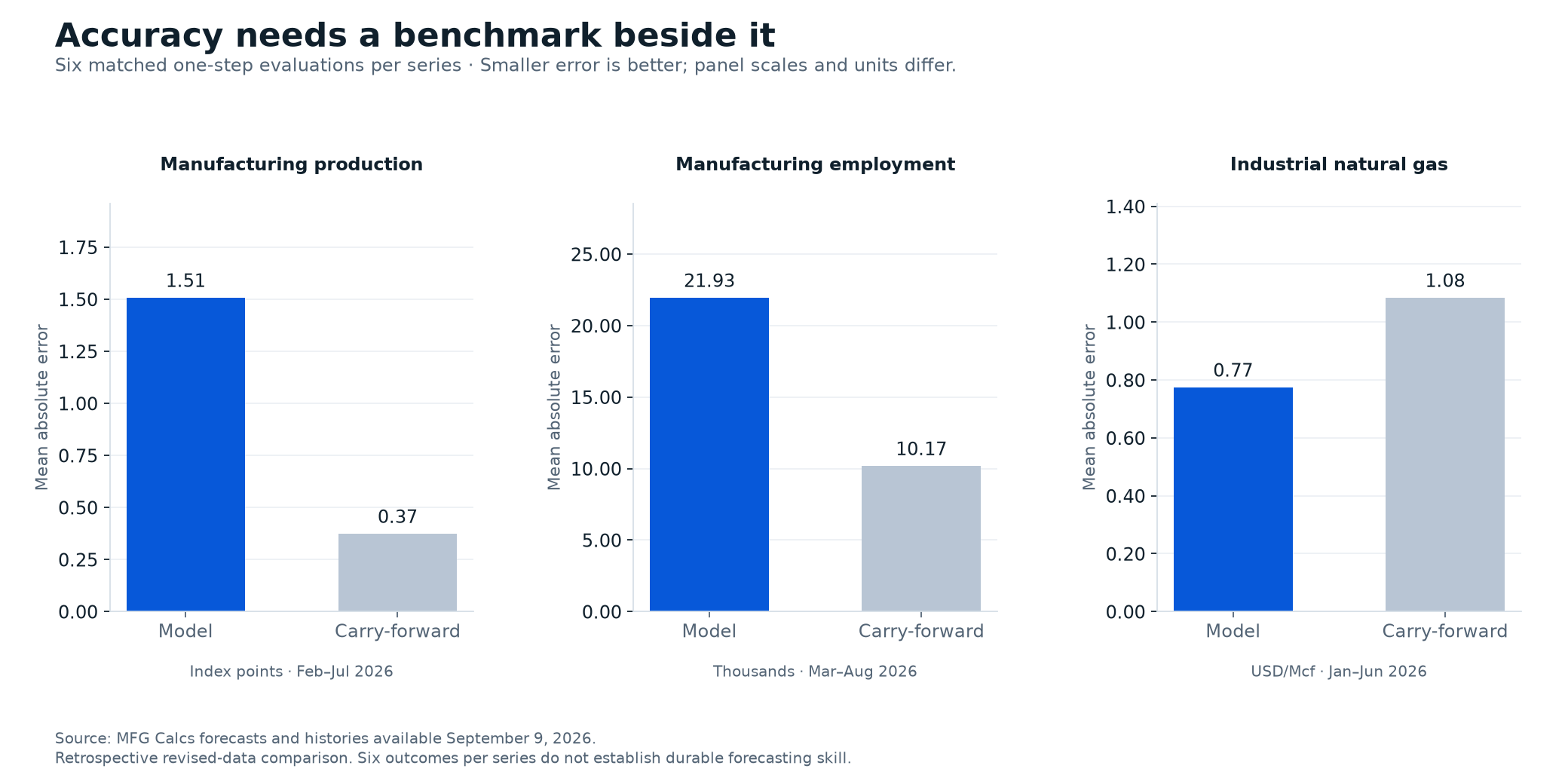
For manufacturing industrial production, the six evaluated observations run from February through July 2026. The model's mean absolute error was 1.51 index points. Carrying forward the preceding month's index produced an error of 0.37 points. Using unrounded inputs, the model's error was 4.04 times the benchmark's. The model also lost this comparison in each three-month half of the period.
The difference is visible in the underlying levels. For April, the saved model prediction was 96.63 and the observed index was 98.76. The previous month's observation, which supplies the benchmark prediction, was 98.07. Both forecasts can look reasonably close on a chart whose scale spans decades of industrial history. They are less similar when judged against the month-to-month movement a planner actually wants to understand.
Manufacturing employment offers a second case. Across March–August 2026, the model's mean absolute error was 21.93 thousand employees, compared with 10.17 thousand for carry-forward. A small error relative to an employment base of millions is compatible with a much larger error than a simple reference forecast. That does not make the employment series useless. It changes what its accuracy statistic can support.
THE MODEL ALSO HAS CLEAR WINS
Industrial natural gas is a counterexample. Across January–June 2026, the model's mean absolute error was $0.77 per thousand cubic feet; carry-forward's was $1.08. The model reduced error by 28.59% using unrounded values. That gain belongs alongside the unfavorable production and employment comparisons.
The distribution matters as much as the examples. Tariff signals accounted for 58 of the 111 eligible series, with 38 beating carry-forward. Across the remaining 53 series, 17 won. Within factory demand, only one of eight did better; within materials and producer prices, five of 16 did. These are descriptions of this evaluated panel. The categories are not equally large, their observations are related, and the counts are not independent trials of forecasting skill.
Changing the simple reference also changes the verdict. We repeated the calculation using the same month one year earlier as the prediction, a seasonal-naive benchmark. The models beat that rule in 89 of 111 series. Only 47 beat both simple alternatives. A favorable comparison against one weak reference cannot establish superiority over another reference that fits the series more closely. Benchmark selection belongs in the published methodology, where readers can inspect it.
SIX MONTHS CANNOT CARRY A PERMANENT VERDICT
We split each series' six observations into two three-observation halves. The models beat carry-forward in 69 series in the first half and 33 in the second. Just 25 won in both. This is a sensitivity check on a small sample, not a formal stability test. Three outcomes can change a ranking sharply, particularly for a volatile series.
Natural gas illustrates the problem within a winner. Its model performed better over all six observations and in the first half, but carry-forward had the smaller error in the second half. Publishing only the favorable six-month average would hide that reversal. Publishing only the unfavorable second half would be equally selective. Both belong beside the full-period result.
The eligible series also cover different calendar windows because their source agencies publish at different speeds. Production ends in July, employment in August, and gas in June. We used the history saved by September 9, 2026 for both the benchmark and the model evaluation. That makes the comparison reproducible within this snapshot, but it is not a reconstruction of every number available to a forecaster on each historical release date. Such a test requires archived publication vintages.
WHAT A MORE DEMANDING SCORECARD WOULD SHOW
An informative scorecard would give readers the model error, the carry-forward error, the seasonal-naive error, the evaluation dates and the number of observations. It would show where a model wins and where it loses, keep the horizon explicit, and separate a backward-looking evaluation from a ledger of forecasts actually published before outcomes arrived. The site's existing forecast charts supply part of that evidence; this comparison supplies a missing reference point.
For this audit, 113 published forecasts in the September 9 snapshot were considered. Two lacked six matched evaluation observations and were excluded: the two retail fuel series. The final panel contains 666 matched forecast/outcome observations, with no duplicated series-month keys and no discrepancies between the scored actual values and their saved history entries. The publication gate already rejects models whose held-out average percentage error exceeds 35%. This is therefore a panel selected partly for accuracy on that same evaluation segment, not a census of every candidate model.
The investigation leaves a specific question for the next release: does each model continue to add information beyond the simple alternatives, across enough observations and the horizons readers use? Until that record is longer, the evidence supports a conditional conclusion. Some forecasts improved on a plain reference during these windows. Many did not. Readers deserve to see that comparison before a small headline error becomes a reason to trust a projection.
SOURCES AND REPRODUCIBLE METHOD
The calculations use the MFG Calcs forecast history preserved in the September 9, 2026 repository snapshot and held-out predictions, with the source period attached to each series. The production example derives from the Federal Reserve manufacturing production series; the gas example uses EIA industrial natural-gas prices. Full per-month actuals, model predictions, benchmark predictions and error calculations accompany this local draft. The analysis uses an evaluation-period error ratio; it is not the separately defined mean absolute scaled error, and it makes no claim of statistical significance or future guaranteed performance.
Sources and evidence
Evidence period: Historical evaluation saved by September 9, 2026. Production: February–July 2026. Employment: March–August 2026. Industrial natural gas: January–June 2026.. The frozen evidence record lists the source files and verified hashes available September 9, 2026. Source revision: 5e4fb7726c3d40060c0151c086c903baae856cab. Later live-data updates do not alter the historical evidence in this article.
fred.stlouisfed.org/series/IPMAN
eia.gov/dnav/ng/ng_pri_sum_dcu_nus_m.htm
Published 2026-09-29.