Manufacturing Costs
One 90-day quote policy covers steel and machinery. Their historical price exposure differs almost tenfold.
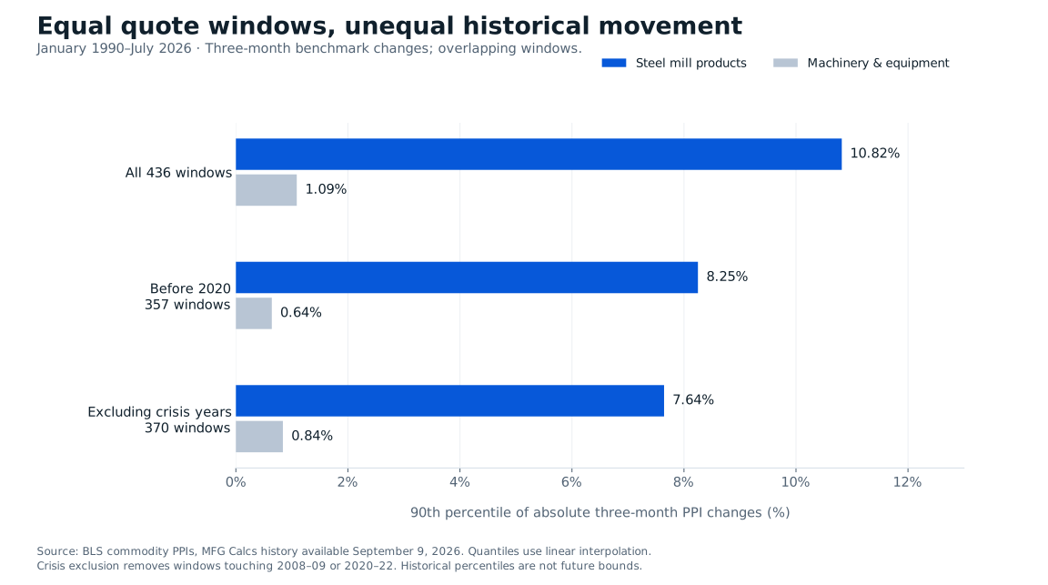
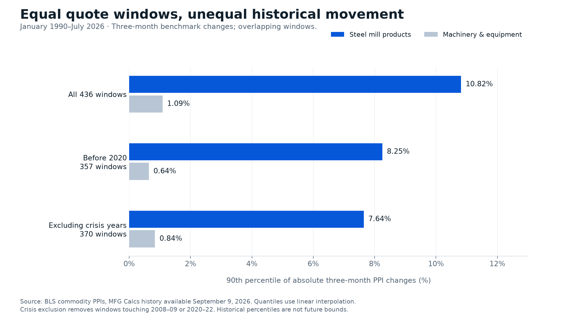
Across 436 three-month windows ending April 1990 through July 2026, steel had a 10.82% 90th percentile absolute change and machinery 1.09%. Removing 2008 to 2009 and 2020 to 2022 leaves 7.64% and 0.84% over 370 windows.
Editorial evidence cutoff: September 9, 2026. Published September 29, 2026. Observation periods are stated throughout; older figures are retrospective evidence.
A 90-day quote can sound like a standard administrative term. The price exposure underneath it is anything but standard. In 36 years of monthly data, the 90th percentile absolute three-month move in the steel mill products price index was 10.82%. For machinery and equipment, it was 1.09%.
That difference is almost tenfold. It does not establish what a supplier should charge, but it challenges the assumption that the same validity window creates comparable exposure across purchasing categories. The relevant question is what can move, how far it has moved over the actual interval, and who absorbs that movement.
For a September 2026 purchasing review, the earlier price episodes offer a practical test of whether a shared quote-validity rule fits the materials being purchased.
View full-size chart
Scroll horizontally to read every label. Keyboard users can focus the chart area and use the arrow keys.
The same deadline covers very different markets
The comparison uses 13 producer-price categories, each with 439 monthly observations from January 1990 through July 2026. For each category, we measured every three-month endpoint change, producing 436 overlapping windows. Three monthly intervals approximate a quarter; they are not exactly 90 calendar days.
Steel exceeded a 5% move in either direction in 127 of those windows. Machinery exceeded that threshold in none. Lumber did so in 126. These counts describe broad domestic selling-price benchmarks, not the number of individual supplier quotations that changed or the frequency of losses on a purchasing contract.
The difference still matters for administration. A single review interval can be sensible for workflow while remaining poorly matched to price exposure. The mistake comes when procedural consistency is treated as evidence that every category needs the same contingency or the same type of adjustment clause.
The dramatic examples are real, and insufficient
Steel's largest observed three-month increase was 49.13%, from January to April 2021. Machinery's largest was 3.28%, from December 2025 to March 2026. The largest steel decline over a three-month window was 24.82%, from September to December 2008.
Selecting those extremes alone would make a forceful chart and an incomplete investigation. The pandemic and financial crisis are not ordinary purchasing environments. A risk discussion that relies exclusively on those episodes can turn a real historical event into a permanent justification for an unnecessarily large price buffer.
That is why the main comparison uses a distribution rather than only a maximum. The 90th percentile absolute move puts upward and downward changes on a common scale. It asks how large a movement was near the upper end of the observed range, while keeping the direction available for a separate contractual discussion.
Remove the shocks and the gap remains
Before 2020, steel's 90th percentile absolute three-month move was 8.25%, compared with 0.64% for machinery. That check contains 357 windows and excludes the pandemic era entirely. The broad difference was already present.
We then removed windows touching either 2008 to 2009 or 2020 to 2022. Among the remaining 370 windows, the steel figure was 7.64% and machinery's was 0.84%. Lumber's corresponding value was 7.49%. Exceptional events enlarged the full-sample numbers, but did not create the basic contrast.
This result supports category-specific review, not a universal percentage cap. A broad machinery index can smooth very different movements in machine tools, engines, pumps or other equipment. A supplier making a particular product may face a cost pattern unlike the aggregate. The next step is to investigate that difference, rather than assume the benchmark settles the negotiation.
A historical tail is not a supplier's entitlement
Suppose a supplier cites steel volatility when requesting an adjustment on a finished assembly. The index history establishes that steel prices have moved substantially over a quarter. It does not establish how much unpurchased steel remains in that order, whether the supplier already fixed its cost, or what share of the finished price the steel represents.
Those distinctions determine the actual exposure. Material already bought at a known price differs from material still to be ordered. A high steel content differs from a labor-intensive assembly. A fixed selling price can also include a deliberate risk premium that must be compared with the cost of alternative terms.
Nor does a quieter machinery index prove that every supplier request above its trailing change is padding. Individual designs, electronics, engineering work and delivery commitments are not identical to an economy-wide basket. The data is most useful as a prompt for a documented cost explanation.
Downward moves deserve the same scrutiny
Using absolute changes reveals the size of movement without privileging one side of the contract. The steel record includes sharp increases and sharp decreases. A clause designed around actual benchmark movement needs to explain how both directions are handled, where appropriate to the commercial agreement.
The base month matters as much as the category. If a quote is signed today but its reference index is several months old, the apparent 90-day exposure contains an additional period. Publication lag, adjustment dates and thresholds can change the practical result even when two clauses name the same PPI.
The steel history and machinery history make those reference points visible. The reader should be able to reproduce the adjustment from two identified observations, rather than reverse-engineer an undefined inflation allowance after the invoice arrives.
Make the review rule fit the purchase
A useful purchasing review starts with the part of the cost still exposed, then chooses a product-relevant benchmark and the time interval actually at risk. Only then does it evaluate historical movements, commercial alternatives and the cost of fixing the price. Starting with a default contingency reverses that order.
For some purchases, a short quote expiry may be workable. For others, a documented adjustment mechanism or a fixed price may be worth more than a small initial discount. The data cannot select among those options without supplier terms and the buyer's operational needs.
It can expose a weak assumption: three months does not mean the same price risk everywhere. The most defensible rule is one whose category, horizon and exposed cost can be explained. That gives the purchasing team something more useful than a dramatic commodity chart, a question the supplier can answer with evidence.
Sources and calculation
The study uses saved BLS producer-price histories, January 1990 to July 2026. Three-month change equals ending index divided by the index three months earlier, minus one. Every history was checked for monthly continuity. Quantiles are descriptive and overlapping windows are dependent. Product labels follow BLS definitions; the broad nonferrous and paper series must not be renamed as narrower finished products.
Sources and evidence
Evidence period: January 1990 to July 2026. The frozen evidence record lists the source files and verified hashes available September 9, 2026. Source revision: 5e4fb7726c3d40060c0151c086c903baae856cab. Later live-data updates do not alter the historical evidence in this article.
data.bls.gov/timeseries/WPU1017
data.bls.gov/timeseries/WPU1025
data.bls.gov/timeseries/WPU1022
data.bls.gov/timeseries/WPU066
data.bls.gov/timeseries/WPU101
data.bls.gov/timeseries/WPU081
data.bls.gov/timeseries/WPU061
data.bls.gov/timeseries/WPU0913
data.bls.gov/timeseries/WPU1015
data.bls.gov/timeseries/WPU1081
data.bls.gov/timeseries/WPU0623
data.bls.gov/timeseries/WPU0653
Published 2026-09-29.